This is the first of many series on machine learning.
Get the Dataset
-
Download the following zip files
-
Unzip the folder and copy
Files and Dataunder folder locationMachine Learning A-Z Template Folder\Part 1 - Data Preprocessing
Review the dataset
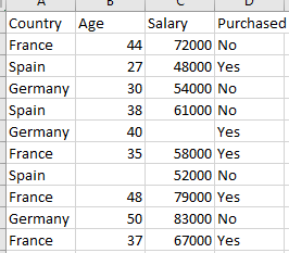
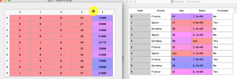
The above dataset shows Country, Age, Salary and Purchased. The field that we need to research is called Dependent field and others are called Independent Field
Dependent Field
A dependent field is a whose outcome or value is derived from other fielda. In this example, we are trying to find Whether a customer made a purchase or not. Hence, Purchased here becomes the dependent field. In terms of coordinate, if we map this on the graph then Purchased will be plotted on the y-axis.
Independent field
Independent fields are values that we observe. Example - If I stand on the side of the freeway and start noting down the color of each car passed, whether it is a car or a truck, is it raining that day or sunny? etc. These values are called Independent fields. In the above datasheet, Country, Age and Salary are independent fields.
In data science, everything is a function. Hence if Purchased field = Y and Country, Age and Salary can be represented as c, a & i respectively. Then the above function can be represented as
Y = Xc + Ta + Zi
Importing the essential library
There are three essential libraries for most basic machine learning projects. Add the below library
import numpy as np import matplotlib.pyplot as plt import pandas as pd
|
|
Import the dataset
Use panadas to import the file data.csv file
|
|
|
|
| Country | Age | Salary | Purchased | |
|---|---|---|---|---|
| 0 | France | 44.0 | 72000.0 | No |
| 1 | Spain | 27.0 | 48000.0 | Yes |
| 2 | Germany | 30.0 | 54000.0 | No |
| 3 | Spain | 38.0 | 61000.0 | No |
| 4 | Germany | 40.0 | NaN | Yes |
| 5 | France | 35.0 | 58000.0 | Yes |
Create the dependent and Independent Variable matrix of features
|
|
Identify the missing data
In the real world when you are handed a dataset. You will find that a lot of data might be missing. Ex - Row 6 Salary is empty and Row 7 Age is missing in our data.csv
Strategies to handle missing data
- Remove the rows that have missing data. This approach is simplest but will skew our dataset if lots of fields are missing.
- Replace the missing data with Mean
- Replace the missing data with Median
- Replace the missing data with Mode or Frequency
As a general rule of thumb mean and median can be applied to numerical values only. It cannot be applied to alphanumeric or String values. This is where we can use Mode or Frequency.
Taking Care of missing data * (Numerical values)*
Scikit library in python provides a class called Imputer which helps in fixing the missing values using the above strategies.
|
|
In the above code we define a SimpleImputer class object.
imputer = SimpleImputer(missing_values = np.nan, strategy='mean')
The next line imputer = imputer.fit(x[:,1:3]) is telling imputer object on which matrix columns it needs to look for missing value and mark them for filling value as mean
The last line x[:, 1:3] = imputer.transform(x[:, 1:3]) fills in the cells of X matrix that were marked by the imputer.
One thing that I wanted to try was that would happen if I just used imputer.fit(x) and did not provide the columns which actually had the missing values. What happens is that since you have marked the strategy as strategy='mean', the imputer will try to take the average/mean of each row country, Age & Salary. Since Country is of type String, python will shit in its pant and complain about it. However, if the Country column was numeric, then this imputer.fit(x) would have worked. Additionally, on the left side we have defined that data be copied into x[:, 1:3]. This is because if you write x = imputer.transform(x[:, 1:3]), imputer has marked the cell to be transformed is (1,5) as there are two columns it is looking at Age and Salary but if put only x on the left side, then (1,5) refers to Age 40, while imputer is expecting it to be a Salary column.
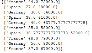
As you can see, the imputer has filled in the missing values for Salary as $63777.78 and Age as 38.7.
Taking care of Categorical data
Categorical data is any data that is not numeric. Think of it as attributes of an object. Ex - If I am observing cars on a freeway and noting down the speed at which the car is driving and the color of the car. The cars may have different colors such as red, green, blue etc. I can only observe them but cannot do anything else with them like add, subtract, find mean or anything. However, a machine learning algorithm may see value in finding a relation between dependent and independent feature. The algorithm can only make use of item if it is defined in numbers.
One way to define them is by assigning them numbers ex- Red =1, Blue =2 and so on.
In our current example, we have a categorical data - Country. To convert or encode as it is called in ML, we will again use a library from Scikit
|
|
array([[0, 44.0, 72000.0],
       [2, 27.0, 48000.0],
       [1, 30.0, 54000.0],
       [2, 38.0, 61000.0],
       [1, 40.0, 63777.77777777778],
       [0, 35.0, 58000.0],
       [2, 38.77777777777778, 52000.0],
       [0, 48.0, 79000.0],
       [1, 50.0, 83000.0],
       [0, 37.0, 67000.0]], dtype=object)
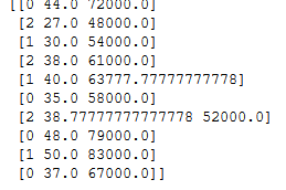
The above code uses LabelEncoder class to encode the values of the country. Here, France =0, Spain = 2, Germany=1
There is however a simple problem here.
#####Problem:
The models are based on equation. Since the LabelEncoder here, has assigned them values 0,1,2, the equation would think that Germany has higher value than France and Spain has a higher value than Germany. This certainly is not the case. These are supposed to be treated as observational values. Example - Picking on our earlier example of observing car speeds and color. If we use LabelEncoder for encoding car colors, the model may come back and say that A red Prius will always be faster than a White Ferrari
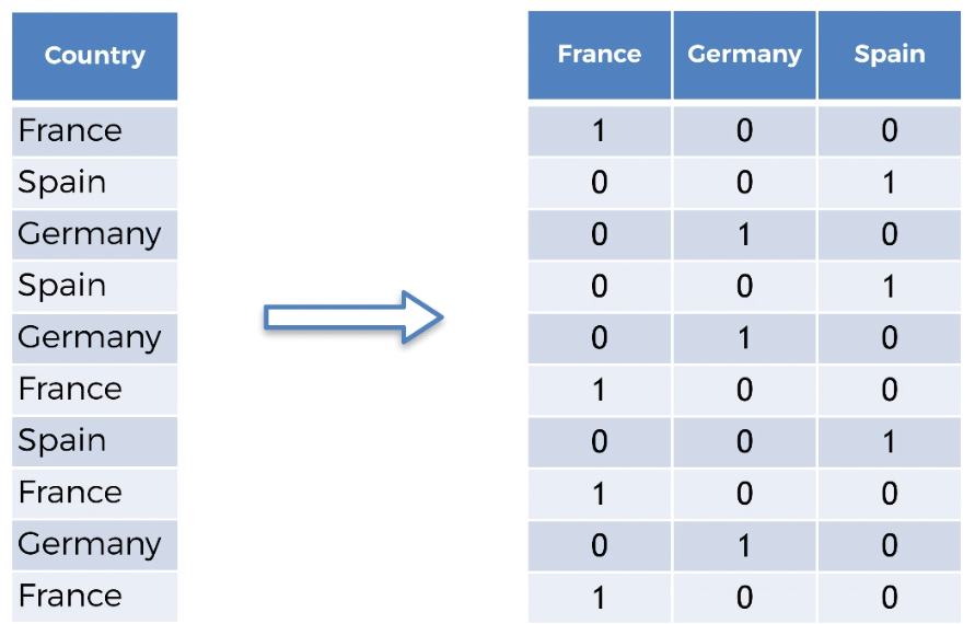
To get over this problem and use category as markers, we will use another class which will create dummy encoding and this gives equal value to all categorical data. It does that by creating a sparse matrix.
|
|
So after dummy encoding, the complete sparse matrix of x looks like this
So now let’s convert the dependent column Purchased as well. However, we do not need to use dummy encoding as there are only two variables and that it is a dependent variable.
|
|
Splitting dataset into training and test set
-
Why do we need to split the data into training and test set?
-
This is about an algorithm that will create the equation to predict the result of new information based on history. If you let it run on all of the data then it will learn too much and will have correlation value or in other words overfitting. A simple example in the real world is of a boy who memorizes the book word by word but fails in the actual exam because instead of asking what is 2 +2 like he read in the book, the exam asked what is 1+3. The student learnt too much but cannot relate or imply the same knowledge on a new data set.
-
Sometimes you may have limited data to build the model and may not additional data to test your model.
-
-
** What is a good ratio to split the data?**
Usually, 80/20 or up to 70/30 is a good number. Going beyond 70/30 is not recommended.
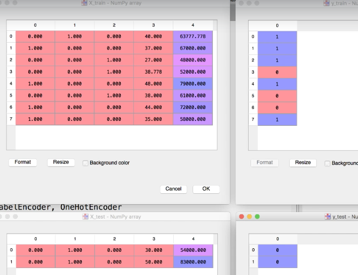
To split a dataset into training and test set. We will use another class called train_test_split, which returns 4 different values - Training_X, Test_X,Training_Y, Test_Y
|
|
The data is now split into 8 and 2 observation.
Feature Scaling/ Normalization/Standardization
If you look your dataset and pay attention to independent features Age and Salary, the range varies for Age between 27 - 50 and Salary between 48000 - 83000. When an equation is created, the distance between two dat apoints is huge and the values can be skewed because one of the columns have 27 for age and 83000 for salary.
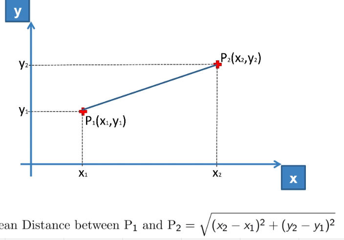
The models are usually based on Euclidean distance. In our case since Salary has a higher range, it will dominate the age values which means when we do distance between observation (27, 48000) and (48, 79000) then (x2-x1) ^2 vs (y2-y1) ^2 is
441 vs 961000000. Hence Age is overshadowed by Salary.
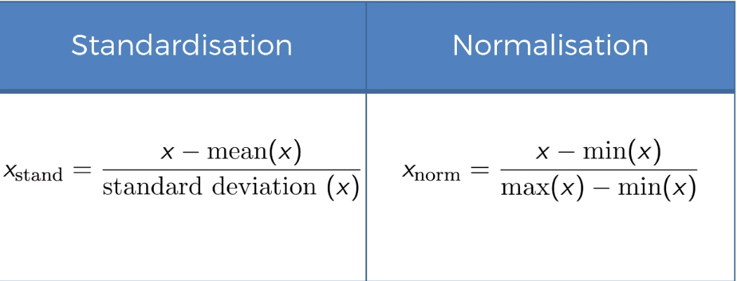
If you are from statistics field, you probably are already familair with standardization or Z-index etc. Above is the two way to calculate the standard range which will always give us a value between 0 and 1
|
|
NOTE: We are not fitting and transforming the x_test because it is already fitted based on xtrain so that they are now on the same scale. If we would have used fit_transform on both test and train then their scale would have been different say one could between -1 and +1 while the other could be on -3 and +3

- Why did we not apply feature scaling on
yor dependent variable?
In this case, the values are 0 and 1 only or in other words, this is a classification problem which has two choices, whether a customer bought the product or he did not buy the product. In other scenarios such as that related to multiple regression, we may have situation where we may have to do feature scaling onyas well.
That’s all for the first series. Stay tuned for next series.